The basic command for sketching the graph of a real-valued function of one variable in MATHEMATICA is
which will draw the graph of y=f(x) over the closed interval [xmin,xmax] on the x-axis. More generally
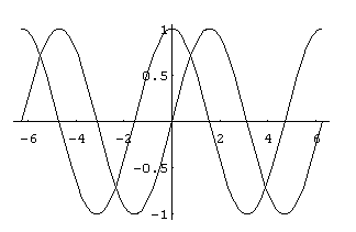
will represent in one picture the graphs of y=f1(x), y=f2(x), ... over the closed interval [xmin,xmax] on the x-axis. For example the output of
is:

To get a fancier output we might add some modifiers such as
obtaining:

Here is a table describing some of the most useful modifiers for the PLOT command.
| AspectRatio -> NN | control aspect ratio (proportions) of viewing window |
| PlotRange -> {NN,NN} | set the height of the window |
| Axes -> BB | include axes or not |
| AxesLabel -> {"xlabel","ylabel"} | label the axes |
| PlotLabel -> "text for title" | put title on graph |
| Background -> Hue[NN] | color the background |
| PlotStyle -> {{s1},{s2},...} | set the color and the "style" of curves |
| GridLines -> Automatic | add grid lines to graph |
In this table, NN denotes a numerical value (which should be between 0 and 1 for Hue[NN]). The symbol BB can be one of the values True or False. And s1 may include specifications such as Hue[NN] (setting curve color), AbsoluteThickness[NN] (setting curve thickness), or Dashing[{NN,NN}] (making the curve dashed). The modifier AspectRatio->Automatic gives the visually true proportions (where the x- and y-axes are scaled equally).
Instead of Hue[NN], colors can also be specified with RGBColor[NN,NN,NN]. Desired colors may be previewed and chosen using the "Color Selector" from the "Input" menu.
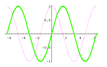
To illustrate the "PlotStyle" modifier, the input
will result in:

If we want to add a frame to this picture, on the next input we could enter Show[ %, Frame->True ]. The effect of the "Show" command is to redraw the graphic (in this case the graphic in the previous output %) with the additional modifier Frame->True.

URL: http://math.ou.edu/~amiller/math/plot.htm
August, 1999