On this page we describe the MATHEMATICA commands ParametricPlot and ParametricPlot3D which can be used for plotting parametrically defined curves in 2- and 3-dimensions. We start with the command for sketching planar curves:
This will draw the curve described by the parametric equations { x = x(t), y = y(t) } as t ranges through the interval [tmin,tmax] . As with the Plot command, two or more curves can be plotted with
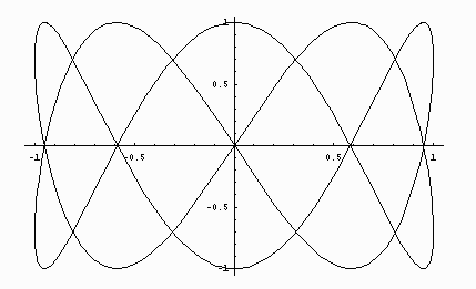
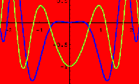
For example the output of
is:

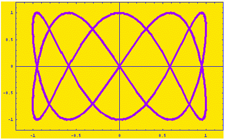
To get a fancier output we might add some modifiers such as
obtaining:
Some of the most useful modifiers for the ParametricPlot command are:
| AspectRatio -> NN | control aspect ratio (proportions) of viewing window |
| PlotRange -> {NN,NN} |
set the dimensions of the viewing window |
| Axes -> BB | include axes or not |
| Frame -> BB | include frame or not |
| AxesLabel -> {"xlabel","ylabel"} | label the axes |
| PlotLabel -> "text for title" | put title on graph |
| Background -> Hue[NN] | color the background |
| PlotStyle -> {{s1},{s2},...} | set the color and the "style" of the curve |
| GridLines -> Automatic | add grid lines to graph |
In this table, NN denotes a numerical value (which should be between 0 and 1 for Hue[NN]). The symbol BB can be one of the values True or False. And s1 may include specifications such as Hue[NN] (setting curve color), AbsoluteThickness[NN] (setting curve thickness), or Dashing[{NN,NN}] (making the curve dashed). The modifier AspectRatio->Automatic gives the visually true proportions (where the x- and y-axes are scaled equally). Instead of Hue[NN], colors can also be specified with RGBColor[NN,NN,NN]. Desired colors may be previewed and chosen using the "Color Selector" from the "Input" menu.
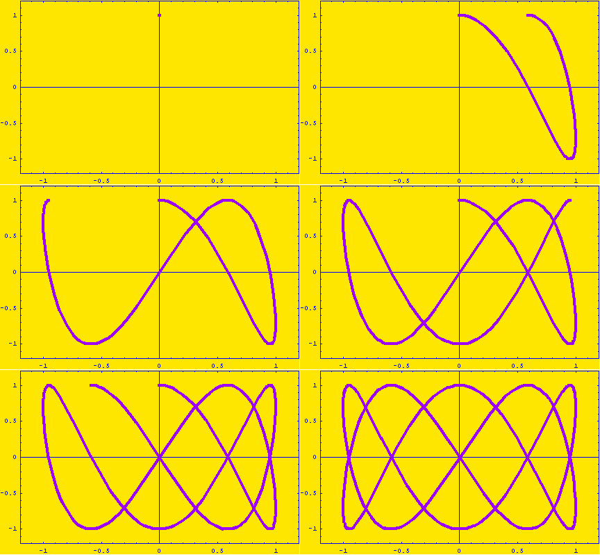
MATHEMATICA can also animate graphics to represent the motion of a parametrization. For example:
  Table[
    ParametricPlot[{Sin[2t], Cos[5t]}, {t, 0, I},
      PlotStyle -> {Hue[.77], Thickness[.01]},
      PlotRange -> {{-1.2, 1.2}, {-1.2, 1.2}}, Frame -> True,
      Background -> Hue[.15]],
  {I, 0, 2*Pi, 2*Pi/20}]
will result in the animation
Or check out this more intricate example plotting two curves simultaneously.
The basic command for sketching a parametrized 3-dimensional curve is:
which draws the curve described by the equations { x = x(t), y = y(t), z = z(t) } as t ranges through the interval [tmin,tmax] .
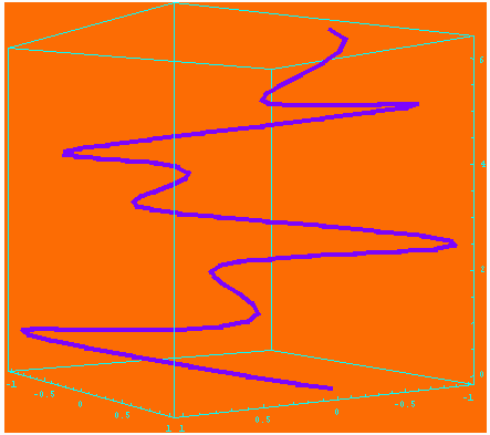
Here's an illustration:
  ParametricPlot3D[
    {Sin[2t], Cos[5t],t,{Hue[.75], Thickness[.01]}}, {t,0,2*Pi},
    BoxRatios->{1,1,1},ViewPoint->{2, 3, 0},
    Background->Hue[.07]   ]
which results in
The modifiers for ParametricPlot3D are similar to those for ParametricPlot with a few variations:
| BoxRatios -> {NN,NN,NN} | control aspect ratio (proportions) of viewing window |
| PlotRange -> {NN,NN,NN} |
set the dimensions of the viewing window |
| ViewPoint -> {NN,NN,NN} | establish the viewpoint for looking at the 3-dimensional plot |
3-dimensional pictures can be hard to interpret at times, it may help to spin the picture in order to gain perspective. Here's a spinning example to illustrate.
URL: http://math.ou.edu/~amiller/math/pplot.htm
November, 1999